For dealing with road/city networks, refer to Geoff Boeing’s blog and his amazing python package OSMnx. Go to Shapely for manipulation of line segments and other objects in python, networkx for networks in python and igraph for networks in R.
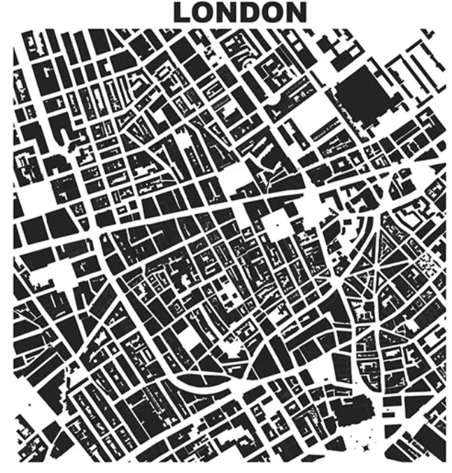
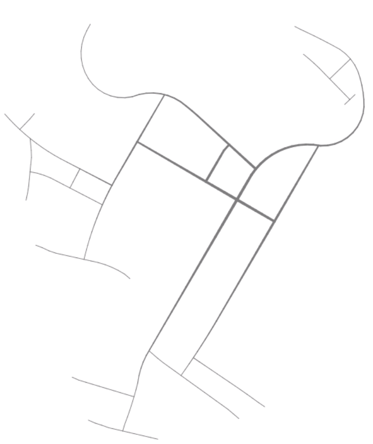
Procedural generation of road networks is normally based on tenor fields but simpler algorithms involving randomly growing roads with an equal probability of splitting into a T-junction or branching a road to the side also make for good results. In particular, I love the work of Oleg Dolya on his Village generator and his twitter post with this graphic:
Selenium Webdriver is a framework that can help you automate browser-related activities (e.g. for testing, scraping). You can emulate user behavior, screenshot, etc. First install selenium on a computer and then the language bindings (python bindings are available).
Phase is important in the perception of speech quality. For stationary GPs, I read that phase might just be uniformly distributed on a circle.
Many real life networks are fat tailed (in terms of the degree distribution).
Causality can be studied from observational data by the assumption of a graph. For example, in the additive noise model, I believe that we assume a graph that looks like \(X \rightarrow Y\) if \(Y = f(X) + \epsilon\) or vice versa. The model is unidentifiable when f is linear and \(\epsilon\) is gaussian.
Information criteria aren’t a good choice while optimizing hyperparameters of certain nonparametric models as they assume that data is conditionally independent given the parameters.
The error term of a statistical model can be (for example a GP) - the aim here is to account for the unmodelled dynamics of a problem and reduce confounding between those and the core model.
Something I was pointed to today: Regression Dilution. Noise in a covariate causes a bias of the slope towards zero. The covariate is dispersed without a change in y values, which causes the regression line to flatten.
An interesting statement: “neural networks use finitely many highly adaptive basis functions whereas gaussian processes typically use infinitely many fixed basis functions” - paraphrased from Wilson et al. 2015, based on work by MacKay, Neal and others.
Many models, particularly those that generate multi-modal posteriors are unidentifiable. Unidentifiability happens when different sets of parameters can produce models whose observations look the same.
Weakly informative priors are better than non-informative ones as they constrain the space enough so that an algorithm searching for the posterior will find it quickly. Strong priors can add a lot of information to a well specified model.
The bootstrap is related to the idea of sampling from an ECDF.
If two random variables \(X\) and \(Y\) are related as \(Y = g(X)\), where \(g\) is a differentiable non-monotonic (but piecewise monotonic) function, and if the density of \(X\) is known to be \(p_X\), then the density of \(Y\) can be expressed as:
\[p_Y(y) = \sum_{x_i \in g^{-1}(y)} p_X(x_i) / \left| \frac{dg}{dx}(x_i) \right|\]… where the sum is over all values \(x_i\) in the preimage set corresponding to \(y\).
One can produce multimodal distributions using monotonic transformations of r.v.s (e.g. normalizing flows).
\(ln \Gamma\) has a left skew whereas \(ln lgN\) is symmetric.
Multivariate normal graphs can be factorized sometimes, when the precision matrix (containing partial autocovariances) is sparse. It’s also possible to discover the direction of certain dependencies in some circumstances.
One way to prove the distribution of SDEs is to solve the Fokker-Planck equation.
The Fourier transform of a covariance function yeilds the spectral density.
Polynomial interpolation (i.e. Lagrange polynomials) can have messy oscillation in higher degrees. This is Runge’s phenomenon and is a similar occurrence to the Gibbs phenomenon in Fourier series on steps.
Independence of cumulants is characteristic of the Normal, and in general, cumulants are not independent.
Uncertainty quantification breaks up a function into orthogonal components and uses this form to calculate moments of r.v.s transformed by this function.
The exponential family is an example of a maxent family of distributions with differing constraints. Moreover, the exponential family is characterized by sufficient statistics with non-increasing lengths w.r.t. the data.
The space of monotonoic and/or positive functions isn’t closed under linear transformations, so it cannot be a vector subspace endowed with a basis! However, there can exist bases (e.g. using the Aitchison geometry) on simplexes, etc. - which aren’t euclidean spaces and the operators defined in these spaces are quite weird.
A model is an idealisation or a description of something. It is a collection of random variables connected by distributional assumptions.
The axioms of probability are disconnected from the interpretation of probability (many of which seem connected in some way).
Sigma algebras can perhaps be thought of as ‘statements’ which could be posed to the probability measure. The probability measure is interesting as it describes how ones measures the underlying variable (e.g. counting).
Non-Measurable Spaces: Example - the Vitali Set. It’s interesting that the construction of these sets always relies on the axiom of choice.
A lot of ideas in the philosophy of science (e.g. falsification, “strength” of induction, not being able to study hypotheses individually, the inability to separate evidence from theory, simplicity of hypotheses, etc.) have corresponding statistical parallels.
Finitely differentiable GPs are Markovian and have a state-space representation.
GP convolution models pass a GP filter over noise.
Gaussian process on spheres are easy to simulate (e.g. by using arc lengths instead of the usual distance metric in the kernel).
The ICA can disentangle signals:
ICA Code
 library(tuneR)
 library(fastICA)

 mix1 <- readWave("./mixedX.wav")
 mix2 <- readWave("./mixedY.wav")

 wave1 <- mix1@left
 wave2 <- mix2@left

 ica <- fastICA(data.frame(x = wave1, y = wave2), 2, method = "R", maxit = 250, tol = 1e-50, verbose = TRUE)

 writeWave(Wave(ica$S[,1], samp.rate = 32000, bit = 16, pcm = TRUE), "./seperatedX.wav")
 writeWave(Wave(ica$S[,2], samp.rate = 32000, bit = 16, pcm = TRUE), "./seperatedY.wav")
Separated Sample:
To perform efficient MCMC for a r.v. which is a deterministic transform of other r.v.s such that you capture the tail of a distribution well, use subset simulation.
Derivatives of 1d GPs
GP Derivative Covariances (1-D)
#!/usr/bin/env python3

from autograd import numpy as np
from autograd import elementwise_grad as egrad

def K(xi, xj):
    """ Calculates the kernel matrix

    The domain values needn't be the same.
    Currently, the only supported dimension of each value of x is one.

    Args:
        xi: Sequence of domain values corresponding to the points changing over rows.
        xj: Sequence of domain values corresponding to the points changing over columns.

    Returns:
        numpy.array corresponding to the kernel values applied over the grid (xi, xj).
    """
    if type(xi) is not float and type(xj) is not float: # if vectorization is possible:
        xi = xi.reshape(-1, 1) # reshape as a column vector
        xj = xj.reshape(1, -1) # reshape as a row vector
    return np.exp(-np.square(xi - xj)) # return kernel calculation

def dK(xi, xj):
    """ Returns the first kernel derivative matrix w.r.t. the second index

    Args:
        xi: Sequence of domain values corresponding to the points changing over rows.
        xj: Sequence of domain values corresponding to the points changing over columns.

    Returns:
        numpy.array corresponding to the kernel derivative values applied over the grid (xi, xj).
    """
    gradient = np.vectorize(egrad(K, 1)) # element-wise gradient along the second index
    xi = xi.reshape(-1, 1) # xi must be a column vector
    xj = xj.reshape(1, -1) # xj must be a row vector
    return gradient(xi, xj)

def d2K(xi, xj):
    """ Returns the second kernel derivative matrix

    Args:
        xi: Sequence of domain values corresponding to the points changing over rows.
        xj: Sequence of domain values corresponding to the points changing over columns.

    Returns:
        numpy.array corresponding to the second kernel derivative applied over the grid (xi, xj).

    """
    gradient = np.vectorize(egrad(egrad(K, 1), 0)) # two derivatives are taken
    xi = xi.reshape(-1, 1) # xi must be a column vector
    xj = xj.reshape(1, -1) # xj must be a row vector
    return gradient(xi, xj)
Simo Särkkä has shown that GPs can be written as state space models, which are models of the form:
\[\dot {\bf x} = A {\bf x} + B {\bf u} \\ f = C {\bf x} + D {\bf u}\]For the centered Matern GP:
\[A = \begin{bmatrix} 0 & 1 & 0 \\ 0 & 0 & 1 \\ -\lambda^3 & -3 \lambda^2 & -3 \lambda \end{bmatrix}, B = \begin{bmatrix} 0 \\0 \\ 1 \end{bmatrix} \\ C = \begin{bmatrix} 1 & 0 & 0 \end{bmatrix}, D = \begin{bmatrix} 0 \end{bmatrix} \\ u \sim \mathcal N, \; \nu = 2.5, \; \lambda = \sqrt{2\nu}/l\]Python code for Matern SSM-GP Simulation
import numpy as np
import matplotlib.pyplot as plt
from scipy.signal import StateSpace

plt.ion(); plt.style.use("ggplot")

##### MATERN GAUSSIAN PROCESS PARAMETERS

l = np.sqrt(2 * 2.5) / 1.0

a = np.array([[0, 1, 0], [0, 0, 1], [-l**3, -3*l**2, -3*l]])
b = np.array([[0], [0], [1]])
c = np.array([[1, 0, 0]])
d = np.array([[0]])

#### STATE SPACE MODEL INPUTS

u = np.random.normal(size = 1000)
t = np.linspace(0, 10, 1000)
x0 = np.random.normal()

#### SIMULATE SSM

model = StateSpace(a, b, c, d)
t, f, x = model.output(u, t)

#### PLOT

plt.plot(t, x)
2021
Efficient Gaussian Process Computation
Using einsum for vectorizing matrix ops
Gaussian Processes in MGCV
I lay out the canonical GP interpretation of MGCV’s GAM parameters here. Prof. Wood updated the package with stationary GP smooths after a request. Running through the predict.gam source code in a debugger, the computation of predictions appears to be as follows:
Short Side Projects
Snowflake GP
Photogrammetry
I wanted to see how easy it was to do photogrammetry (create 3d models using photos) using PyTorch3D by Facebook AI Research.
Dead Code & Syntax Trees
This post was motivated by some R code that I came across (over a thousand lines of it) with a bunch of if-statements that were never called. I wanted an automatic way to get a minimal reproducing example of a test from this file. While reading about how to do this, I came across Dead Code Elimination, which kills unused and unreachable code and variables as an example.
2020
Astrophotography
I used to do a fair bit of astrophotography in university - it’s harder to find good skies now living in the city. Here are some of my old pictures. I’ve kept making rookie mistakes (too much ISO, not much exposure time, using a slow lens, bad stacking, …), for that I apologize!
Probabilistic PCA
I’ve been reading about PPCA, and this post summarizes my understanding of it. I took a lot of this from Pattern Recognition and Machine Learning by Bishop.
Spotify Data Exploration
The main objective of this post was just to write about my typical workflow and views. The structure of this data is also outside my immediate domain so I thought it’d be fun to write up a small diary working with the data.
Random Stuff
For dealing with road/city networks, refer to Geoff Boeing’s blog and his amazing python package OSMnx. Go to Shapely for manipulation of line segments and other objects in python, networkx for networks in python and igraph for networks in R.
Morphing with GPs
The main aim here was to morph space inside a square but such that the transformation preserves some kind of ordering of the points. I wanted to use it to generate some random graphs on a flat surface and introduce spatial deformation to make the graphs more interesting.
SEIR Models
The model is described on the Compartmental Models Wikipedia Page.
Speech Synthesis
The initial aim here was to model speech samples as realizations of a Gaussian process with some appropriate covariance function, by conditioning on the spectrogram. I fit a spectral mixture kernel to segments of audio data and concatenated the segments to obtain the full waveform.
Sparse Gaussian Process Example
Minimal Working Example
2019
An Ising-Like Model
… using Stan & HMC
Stochastic Bernoulli Probabilities
Consider: