The model is described on the Compartmental Models Wikipedia Page.
I wrote a quick-and-dirty Dash app to eyeball good initial starting values for the parameters.
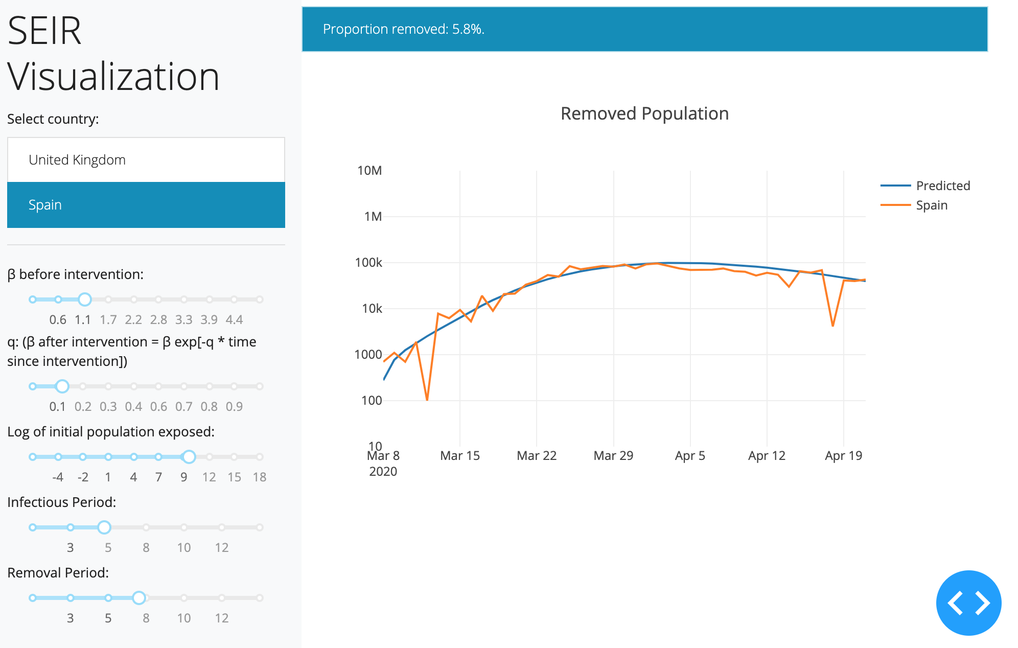
Quick & Dirty Dash App Code to visualize a continuous time SEIR model
import requests
import dash, json
import numpy as np
import pandas as pd
import datetime as dt
from functools import lru_cache
import dash_core_components as dcc
import dash_html_components as html
import dash_bootstrap_components as dbc

from pyswarm import pso
from plotly.graph_objs import *
from scipy.integrate import odeint
from plotly import graph_objs as go
from dash.dependencies import Input, Output

# @lru_cache(maxsize = 3)
def get_data(country = 'Spain'):
    assert country in ['Spain', 'United Kingdom']

    data = requests.get('https://pomber.github.io/covid19/timeseries.json')
    data = pd.DataFrame(data.json()[country])
    data = data.loc[data.deaths >= 10, :]
    data.date = pd.to_datetime(data.date)
    data.reset_index(inplace = True)

    if country == 'Spain':
        lockdown_date = dt.datetime(2020, 3, 15)
    if country == 'United Kingdom':
        lockdown_date = dt.datetime(2020, 3, 24)

    return data, lockdown_date

def dydt(y, t, *args):
    S, E, I, R = y; N = np.sum(y);
    b_0, b_1, a, y, t_l = args
    dxdt = np.zeros(4)

    b = b_0 * np.exp(-b_1 * np.max([0, t - t_l])) # b_0 if t <= t_l else b_1

    dxdt[0] = -b*S*I/N
    dxdt[1] = b*S*I/N - a*E
    dxdt[2] = a*E - y*I
    dxdt[3] = y*I
    return dxdt

def simulate(b_0 = 0.99, b_1 = 0.1, t_l = 50, n = 1e6, e_0 = 10, i_0 = 0, t = 100, infec_prd = 5, recov_prd = 7):
    theta = (b_0, b_1, 1/infec_prd, 1/recov_prd, t_l)
    initial_state = [n - e_0 - i_0, e_0, i_0, 0]
    simuation = odeint(dydt, initial_state, np.arange(t), args = theta)
    return simuation

app = dash.Dash(__name__, external_stylesheets = [dbc.themes.YETI])

app.layout = html.Div(children=[

    html.Div(children=[
        html.H1(children='SEIR Visualization'),

        html.Label('Select country:'),

        dbc.ListGroup([
            dbc.ListGroupItem("United Kingdom", id="country_uk", n_clicks=0),
            dbc.ListGroupItem("Spain", id="country_sp", n_clicks=1)]
        ),

        dcc.Markdown('---'),

        html.Label('β before intervention:'),

        dcc.Slider(
                id='b_0',
                min=0,
                max=5,
                marks={i: 'Label {}'.format(i) if i == 1 else str(np.round(i, 1)) for i in np.linspace(0, 5, 10)},
                value=1.15,
                step=0.01
            ),

        html.Label('q: (β after intervention = β exp[-q * time since intervention])'),

        dcc.Slider(
                id='b_1',
                min=0,
                max=1,
                marks={i: 'Label {}'.format(i) if i == 1 else str(np.round(i, 1)) for i in np.linspace(0, 1, 10)},
                value=0.125,
                step=0.01
            ),

        html.Label('Log of initial population exposed:'),

        dcc.Slider(
                id='e_0',
                min=-7,
                max=np.log(47e6),
                marks={i: 'Label {}'.format(i) if i == 1 else str(int(np.round(i))) for i in np.linspace(-7, np.log(47e6), 10)},
                step=0.01
            ),

        html.Label('Infectious Period:'),

        dcc.Slider(
                id='infec_prd',
                min=1,
                max=14,
                marks={i: 'Label {}'.format(i) if i == 1 else str(int(np.round(i))) for i in np.linspace(1, 14, 7)},
                value=5.1,
                step=0.1
            ),

        html.Label('Removal Period:'),

        dcc.Slider(
                id='recov_prd',
                min=1,
                max=14,
                marks={i: 'Label {}'.format(i) if i == 1 else str(int(np.round(i))) for i in np.linspace(1, 14, 7)},
                value=7.1,
                step=0.1
            )
        ], style = {
            "position": "fixed",
            "top": 0,
            "left": 0,
            "bottom": 0,
            "width": "19rem",
            "padding": "2rem 1rem",
            "background-color": "#f8f9fa",
        }),

    html.Div(children = [

        dbc.Alert(id = "prop-rem", color="primary"),

        dcc.Graph(id='viz-graph')], style = {
            "margin-left": "18rem",
            "margin-right": "2rem",
            "padding": "2rem 1rem",
        })
])

@app.callback(
    [Output("country_uk", "active"),
     Output("country_sp", "active")],
    [Input("country_uk", "n_clicks"),
     Input("country_sp", "n_clicks")]
)
def update_country(ncl_uk, ncl_sp):
    print((ncl_uk, ncl_sp))
    if ncl_uk is None:
        return False, True
    if (ncl_sp is None) or (ncl_sp >= ncl_uk):
        return False, True
    return True, False

@app.callback(
    Output("e_0", "value"),
    [Input("country_uk", "active"),
     Input("country_sp", "active")]
)
def update_initial_exposed(country_uk, country_sp):
    if country_uk:
        e_0 = 9
    if country_sp:
        e_0 = 10
    return e_0

@app.callback(
    [Output("viz-graph", "figure"),
     Output("prop-rem", "children")],
    [Input("country_uk", "active"),
     Input("country_sp", "active"),
     Input("b_0", "value"),
     Input("b_1", "value"),
     Input("e_0", "value"),
     Input("infec_prd", "value"),
     Input("recov_prd", "value")]
)
def update_histogram(country_uk, country_sp, b_0, b_1, e_0, infec_prd, recov_prd):

    if country_uk:
        country = 'United Kingdom'
    if country_sp:
        country = 'Spain'
    data, lockdown_date = get_data(country)

    ifr = 0.01
    n = len(data.deaths)
    t_l = np.argwhere(np.array(data.date == lockdown_date))[0, 0]
    simulated_seir = simulate(b_0 = b_0, b_1 = b_1, t_l = t_l, n = 47e6, t = n, e_0 = np.exp(e_0), i_0 = 0, infec_prd = infec_prd, recov_prd = recov_prd)
    timestamps = data.loc[1:, 'date']
    simulated_removals_diff = np.diff(simulated_seir[:, 3])
    actual_removals_diff = np.diff(data.deaths)

    return {
            'data': [
                {'x': timestamps, 'y': simulated_removals_diff, 'type': 'line', 'name': 'Predicted'},
                {'x': timestamps, 'y': actual_removals_diff/ifr, 'type': 'line', 'name': country},
            ],
            'layout': {
                'title': 'Removed Population',
                'yaxis': {'range': [1, 7], 'type': 'log'}
            }
        }, str('Proportion removed: ' + str(int(1000 - simulated_seir[-1, 0]/47e3)/10) + '%.')

if __name__ == "__main__":
    app.run_server(debug=True, port=8080, host='0.0.0.0')
A Discrete Time SEIR Model in JAGS
This is an implementation of the discrete time epidemiological (SEIR) model based on:
P. E. Lekone and B. F. Finkenstädt, “Statistical Inference in a Stochastic Epidemic SEIR Model with Control Intervention”, 2006.
I’ve made some changes to it, e.g. below, an intervention does not lead to an exponential decay of exposure probabilities - rather, the intervention considered here (a lockdown) just leads to lower exposure probabilities. If the population is large, the paths are very close to the model’s continuous time counterpart (the binomial variance is pretty small), so perhaps the stochastic treatment of the paths (and so many hidden states) isn’t necessary.
JAGS Code
model {
    b_i ~ dexp(1)
    b_m ~ dunif(0, b_i)

    S[1] = N
    E[1] = E_0
    I[1] = 0
    R[1] = 0

    for(t in 1:(T - 1)) {

        S[t + 1] = S[t] - B[t]
        E[t + 1] = E[t] + B[t] - C[t]
        I[t + 1] = I[t] + C[t] - D[t]
        R[t + 1] = R[t] + D[t]

        B[t] ~ dbin(Pr[t], S[t])
        C[t] ~ dbin(1 - exp(-p), E[t])
        D[t] ~ dbin(1 - exp(-y), I[t])

        b[t] = ifelse(t <= T_l, b_m, b_i)
        Pr[t] = 1 - exp(-b[t] * I[t] / N)
    }
}
2021
Efficient Gaussian Process Computation
Using einsum for vectorizing matrix ops
Gaussian Processes in MGCV
I lay out the canonical GP interpretation of MGCV’s GAM parameters here. Prof. Wood updated the package with stationary GP smooths after a request. Running through the predict.gam source code in a debugger, the computation of predictions appears to be as follows:
Short Side Projects
Snowflake GP
Photogrammetry
I wanted to see how easy it was to do photogrammetry (create 3d models using photos) using PyTorch3D by Facebook AI Research.
Dead Code & Syntax Trees
This post was motivated by some R code that I came across (over a thousand lines of it) with a bunch of if-statements that were never called. I wanted an automatic way to get a minimal reproducing example of a test from this file. While reading about how to do this, I came across Dead Code Elimination, which kills unused and unreachable code and variables as an example.
2020
Astrophotography
I used to do a fair bit of astrophotography in university - it’s harder to find good skies now living in the city. Here are some of my old pictures. I’ve kept making rookie mistakes (too much ISO, not much exposure time, using a slow lens, bad stacking, …), for that I apologize!
Probabilistic PCA
I’ve been reading about PPCA, and this post summarizes my understanding of it. I took a lot of this from Pattern Recognition and Machine Learning by Bishop.
Spotify Data Exploration
The main objective of this post was just to write about my typical workflow and views. The structure of this data is also outside my immediate domain so I thought it’d be fun to write up a small diary working with the data.
Random Stuff
For dealing with road/city networks, refer to Geoff Boeing’s blog and his amazing python package OSMnx. Go to Shapely for manipulation of line segments and other objects in python, networkx for networks in python and igraph for networks in R.
Morphing with GPs
The main aim here was to morph space inside a square but such that the transformation preserves some kind of ordering of the points. I wanted to use it to generate some random graphs on a flat surface and introduce spatial deformation to make the graphs more interesting.
SEIR Models
The model is described on the Compartmental Models Wikipedia Page.
Speech Synthesis
The initial aim here was to model speech samples as realizations of a Gaussian process with some appropriate covariance function, by conditioning on the spectrogram. I fit a spectral mixture kernel to segments of audio data and concatenated the segments to obtain the full waveform.
Sparse Gaussian Process Example
Minimal Working Example
2019
An Ising-Like Model
… using Stan & HMC
Stochastic Bernoulli Probabilities
Consider: