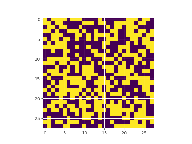
Snowflake GP
Based on the paper:
Learning Invariances using the Marginal Likelihood (2018)
GP with prior that is invariant to sixfold rotation and mirroring.
library(ggplot2)
library(reticulate)
library(data.table)

set.seed(42^2)

cdist = import('scipy')$spatial$distance$cdist

k_g = function(d, s=1, l=1) s*exp(-(d^2) / (l^2))

n = 60
x = cbind(rep(seq(-3, 3, l=n), n),
          rep(seq(-3, 3, l=n), each=n))

R = function(t) matrix(c(cos(t), sin(t), -sin(t), cos(t)), 2, 2)

xs = list()
for (i in 0:5) {
    add_x = x %*% R(i*pi/3)
    xs[[length(xs) + 1]] = add_x
    xs[[length(xs) + 1]] = add_x[, 2:1]
}

S = matrix(0, n^2, n^2)
for(i in 1:length(xs))
    for(j in 1:length(xs))
        S = S + k_g(cdist(xs[[i]], xs[[j]]))

y = as.numeric(t(chol(S + diag(n^2)*1e-5)) %*% rnorm(n^2))

df = data.table(x[, 1], x[, 2], y)
df = df[, .(y = mean(y)), by=.(x_a = factor(V1), x_b = factor(V2))]

ggplot(df, aes(x=x_a, y=x_b, fill=y)) +
    geom_tile() +
    theme(legend.position = "none",
          panel.grid = element_blank(),
          axis.title = element_blank(),
          axis.text = element_blank(),
          axis.ticks = element_blank(),
          panel.background = element_blank()) +
    scale_fill_distiller(palette = "Spectral")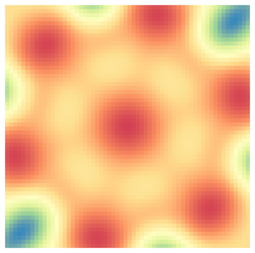
Plotting Google Maps Data
Red is day, blue is night.
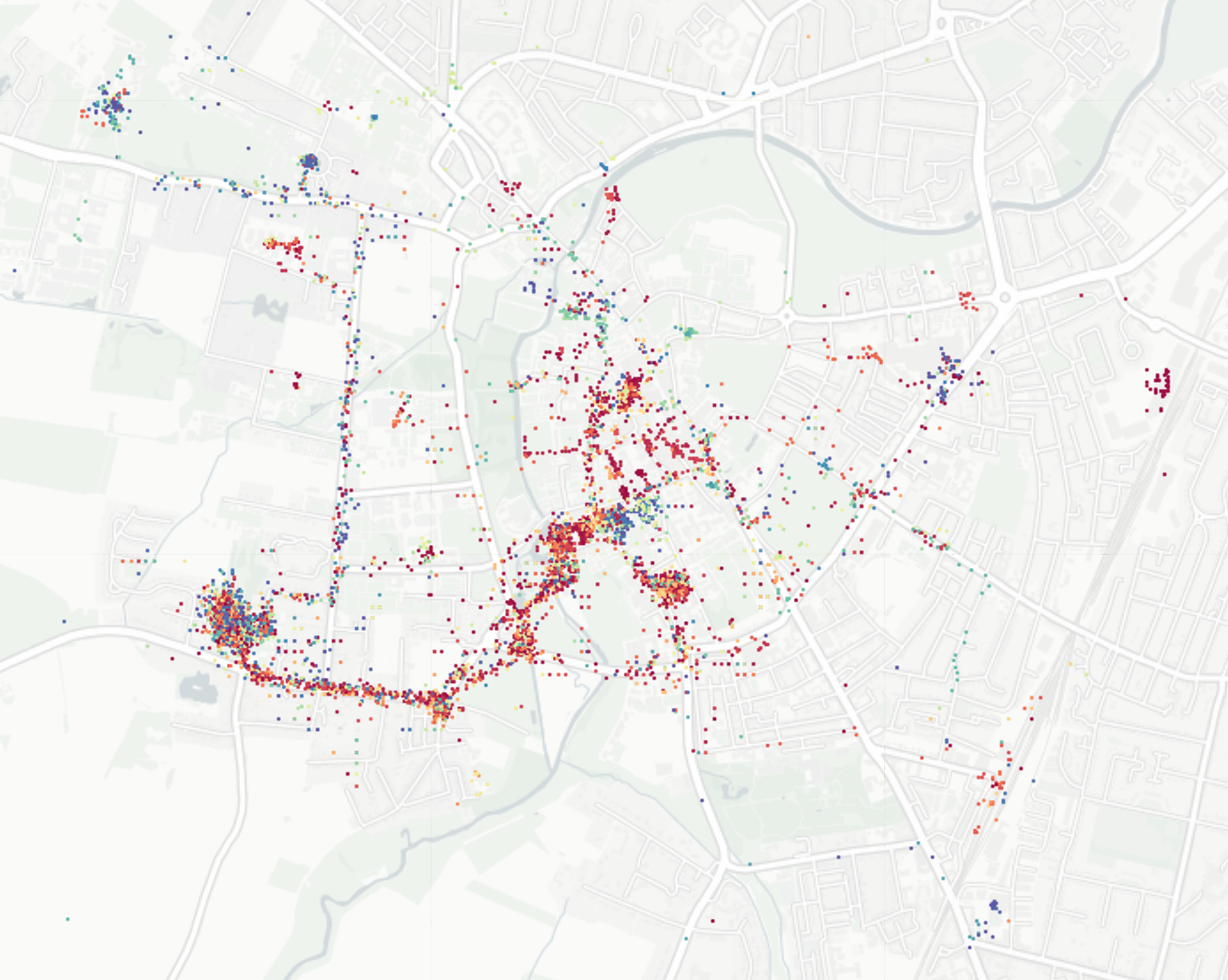
I love the blue mass at the astronomy centre and the movie theatre.
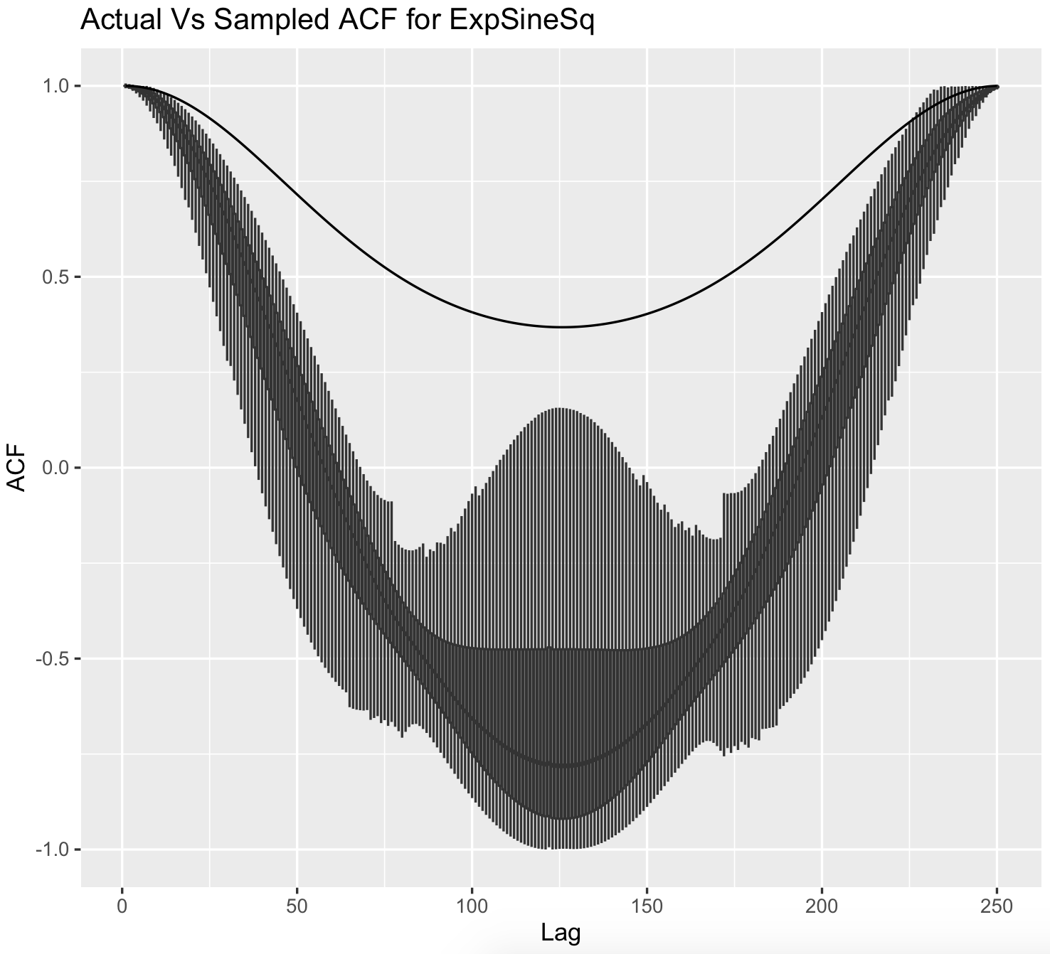
Inferring Gaussian Process Autocorrelation
It seems reasonable and intuitive to think that the sample autocovariance function of a stationary gaussian process would be a sufficient statistic for its covariance function, and I read that this is indeed true for certain stationary GPs with a rational spectrum. This condition is quite similar (if not the same) for GPs to possess a state space representation.
It’s also interesting that not all GPs are ergodic. GPs are mixing (and hence ergodic, I believe) if the covariance dies off to zero after a point, or if its spectrum is absolutely continuous. Loosely, this means that the distribution of the process can be inferred from just one long sample. GPs with an exponentiated sine squared (ESS) covariance function, for example, wouldn’t be ergodic as the spectrum has an infinity at the period.
As a consequence, the covariance function of a zero mean GP with an ESS kernel, and similar signals, cannot be inferred from a single sample. This is reasonable, as no matter how long the signal is, there’s no new information in it after a certain point. Intuitively, a sample from a zero mean GP with an ESS kernel might look like \((3, 2.5, 3, 2.5, ...)\). The ESS is a kernel which is periodic, and the correlation of points spaced half a period apart is closest to zero (compared to any other pair of points), but still strictly positive. Another sample from that GP may look like \((-2, -1.7, -2, -1.7, ...)\).
Points one and two are closer together within each sample than across samples due to the correlation, but given just one observation of the signal (and with no knowledge of the mean of the process), it would appear that points one and two are negatively correlated.
The image below shows this; the black line is the true autocovariance function of the zero mean GP with an ESS kernel, and the boxplots show the sampling distribution of the unbiased sample autocovariance function based on single samples.
Griffin Lim Algorithm and a Minimal Working Implementation
This minimal implementation below is based on the Librosa source on GitHub.
GLA
MWE of the Griffin-Lim:import numpy as np
from scipy.signal import stft, istft
from scipy.io import wavfile as wav
sr, audio = wav.read('audio.wav')
stft_of_audio = stft(audio)[2]
st_spectrum = np.abs(stft_of_audio)
angles = np.empty(st_spectrum.shape, dtype=np.complex64)
angles[:] = np.exp(2j * np.pi * np.random.rand(*st_spectrum.shape)) # angles[:] = 1.0
stft_recon = 0.; momentum = 0.99
for _ in range(2000):
stft_recon_prv = stft_recon
signal_recon = istft(st_spectrum * angles)[1]
stft_recon = stft(signal_recon)[2]
angles[:] = stft_recon - (momentum / (1 + momentum)) * stft_recon_prv
angles[:] /= np.abs(angles) + 1e-16
audio_recon = np.array(signal_recon, dtype = np.int16)
audio_recon = np.repeat(audio_recon, 2).reshape(-1, 2)
wav.write("audio.wav", sr, audio_recon)import numpy as np
from scipy.linalg import dft
np.random.seed(42)
n = 8; n_fft = 4; hop_length = 2; D = dft(n_fft)
x = np.random.normal(size=n)
def stft(x):
n_frames = n//hop_length - 1
stft = np.zeros((n_fft, n_frames), dtype='complex')
for i in range(n_frames):
stft[:, i] = D @ x[(i*hop_length):(i*hop_length + n_fft)]
return stft
S = stft(x)
def istft(stft_matrix):
signal = np.zeros(n)
win_sum = np.zeros(n)
win_sq = np.ones(n_fft)
ytmp = (D.T.conj()/n_fft @ S).real
n_frames = stft_matrix.shape[1]
for frame in range(n_frames):
sample = frame * hop_length
signal[sample : (sample + n_fft)] += ytmp[:, frame]
win_sum[sample : (sample + n_fft)] += win_sq
return signal/win_sum
istft(S) - xThe GLA is an algorithm that tries to recover phase information given a matrix \(X\) which is the absolute value of an STFT. The algorithm minimizes the frobenius norm:
\[|X - S \circ S^{-1} (X)|_F\]where \(S\) is the STFT operation and \(S^{-1}\) is the inverse. The absolute value of \(X\) - the spectrum - must be fixed. This norm is supposed to be zero for “proper” STFTs, but it isn’t when initiated with random phases like in the code above (the STFT has redundant information, so one point may be used in multiple windows - so when initiated with random phases, the matrix might not correspond to anything sensible and may be inconsistent due to the windows overlapping). It is quite interesting to me that, in a probabilistic sense, STFTs of signals would probably only ever admit a density where this norm is zero (i.e. if the STFT was consistent in the overlapping windows). By minimising this norm, we approach an STFT with phases more or less consistent with the spectrum we’ve got, so this “loss” doesn’t correspond to a likelihood.
RL
a. Tic-Tac-Toe Q Learning
I wrote up an implementation of an inefficient table-based Q-learning algo that has a dataframe contain all possible states and future states in tic-tac-toe. The (pretty ugly) code is below. Here, a reward is +1 if x wins, -1 if o wins, 0 otherwise.
Since it’s a solved game, the Qs only take the value -1, 0 or 1 after fitting.
Tic-Tac-Toe Q Learning
import numpy as np
import pandas as pd
from itertools import product

def validate(string):
    blanks = string.count(' ')
    xs = string.count('x')
    os = string.count('o')

    return (blanks + xs + os == 9) and \
           ((xs == os) or (xs - os == 1))

boards = list(map(lambda x: ''.join(x), product(*[' xo'] * 9)))
boards = [board for board in boards if validate(board)]

df = pd.DataFrame(dict(boards=boards))

def event(string):
    x_wins = 0; o_wins = 0

    select = lambda x: ''.join([string[i] for i in x])

    winning_lines = (
        string[:3], string[3:6], string[6:9], # rows
        select([0, 3, 6]), select([1, 4, 7]), select([2, 5, 8]), #cols
        select([0, 4, 8]), select([2, 4, 6]) # diag
    )

    for line in winning_lines:
        unique_chars = ''.join(set(line))
        if len(unique_chars) == 1 and unique_chars != ' ':
            if unique_chars == 'x':
                x_wins += 1
            if unique_chars == 'o':
                o_wins += 1

    if x_wins + o_wins == 1:
        if x_wins: return 'x'
        if o_wins: return 'o'
    elif x_wins + o_wins > 2:
        return 'i' # impossible boards

    if string.count(' '):
        return ''
    else:
        return 'd'

df['event'] = df.apply(lambda x: event(x['boards']), axis=1)
df = df.loc[df.event != 'i'].reset_index(drop=True)

df['Q'] = np.random.uniform(-0.1, 0.1, size=df.shape[0])
df.loc[df.event == 'd', 'Q'] = 0.0
df.loc[df.event == 'x', 'Q'] = 1.0
df.loc[df.event == 'o', 'Q'] = -1.0
df['Q_next'] = df['Q'].copy()

def next_state(string, return_index=True):
    next_char = 'x' if string.count('x') == string.count('o') else 'o'
    chars = tuple(string)
    next_states = [''.join(chars[:i] + (next_char,) + chars[(i + 1):]) \
                   for i in range(9) if chars[i] == ' ']

    if return_index:
        next_states = list(df.loc[df.boards.isin(next_states)].index)
    return next_states

df['next_state'] = None
df.loc[df.event == '', 'next_state'] = \
    df.loc[df.event == ''].apply(lambda x: next_state(x['boards']), axis=1)

def next_q(string, index):
    qs = np.array(df.Q)[df.loc[index, 'next_state']]
    return qs.max() if string.count('x') == string.count('o') else qs.min()

for _ in range(100):
    df.loc[df.event == '', 'Q_next'] =\
        df.loc[df.event == ''].apply(lambda x: next_q(x['boards'], x.name), axis=1)
    df.loc[:, 'Q'] = df.Q*0.9 + 0.1*df.Q_next

df.loc[df.boards == 'xxo o x  ', 'Q'] # expected reward is 0 because it's o's turn
df.loc[df.boards == 'xxo o x o', 'Q'] # expected reward is 1 because the next turn, x wins
b. DnD / Pokemon Battle Simulations
I coded up some classes in python but haven’t gotten around to coding up the RL side of it. One neat trick: as moves can be special and do weird stuff, I coded them up as dicts of metadata, with a field named “special_effects” that contains a lambda function that takes in the opponent class instance and applies the weird stuff to it.
Simulation out of Boredomville
Sometimes one can simplify decisions as other choices may be strictly worse. Then, simple simulation can lead to the probability that a party wins, as a function of input params.sim = function(eagle_hp=26, dragon_hp=22, eagle_ac=13,
dragon_ac=16, eagle_str=3, eagle_dex=3,
dragon_dex=1, dragon_str=2, can_use_bw=T) {
d = function(n=1, r=20) sample(1:r, n, T)
adv = function(roll) ifelse(roll == 20, 2, 1)
eagle_turn = function(ac) {
dmg = 0; hit = d()
if(hit + 2 + eagle_str >= ac)
dmg = dmg + adv(hit)*d(1, 6) + eagle_str
hit = d()
if(hit + 2 + eagle_str >= ac)
dmg = dmg + adv(hit)*sum(d(2, 6)) + eagle_str
return(dmg)
}
dragon_turn = function(ac) {
if(can_use_bw) {
if(sample(0:2, 1)) can_use_bw = F
save_mod = ifelse(d() + eagle_dex >= 11, 0.5, 1)
return(floor(save_mod * sum(d(4, 8))))
}else{
hit = d()
if(hit + 2 + dragon_str >= ac)
return(adv(hit)*d(1, 10) + dragon_str)
else return(0)
}
}
if(d() + eagle_dex >= d() + dragon_dex)
dragon_hp = dragon_hp - eagle_turn(dragon_ac)
while(T) {
if(dragon_hp <= 0) return(1)
eagle_hp = eagle_hp - dragon_turn(eagle_ac)
if(eagle_hp <= 0) return(0)
dragon_hp = dragon_hp - eagle_turn(dragon_ac)
}
}
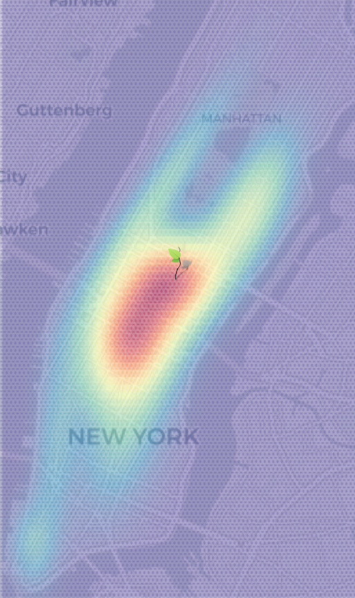
mean(replicate(10000, sim()))New York Conditional Taxi Dropoff Probabilities
I fit a twenty component mixture of multivariate normals, using scikit-learn, to the four dimensional new york taxi pickup/dropoffs dataset.
The dimensions look like (pickup_lat, pickup_lon, dropoff_lat, dropoff_lon). The aim is to predict the distribution of (dropoff_lat, dropoff_lon) by conditioning on (pickup_lat, pickup_lon).
Envelope Modelling
Google’s Quick Draw dataset contains multiple observations of quickly drawn envelopes. I fit a 256-component restricted boltzmann machine to the data, which represents a distribution over the random field that represents an envelope image. Starting off with a completely random image, using Gibbs sampling, we can make our way to the typical set of the distribution, which hopefully looks like an envelope. Here’s what the burn in looks like:
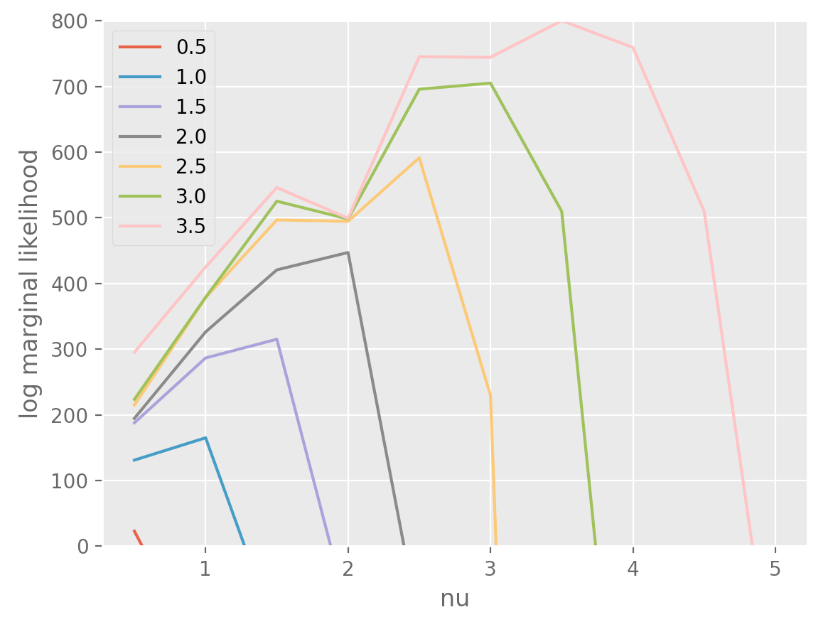
Inferring the Extent of Differentiability
Let’s say that we have an observation of a noiseless function but we don’t know how smooth it is. You could probably fit a Matern GP with different smoothness parameters to see which parameter maximises the log marginal likelihood (the matern parameter corresponds to the number of times one can differentiate a sample from the gp).
Below, I’ve simulated a series from a Matern GP with a particular differentiability parameter, and fit it using differentiability parameters ranging from \(\\{0.5, ..., 5\\}\). The color & label correspond to the parameter while sampling.
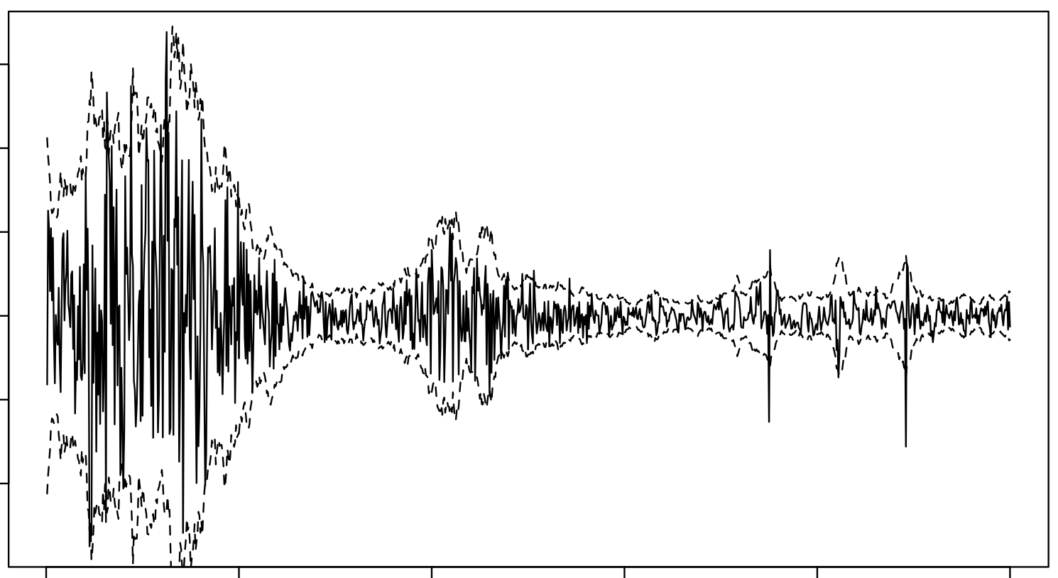
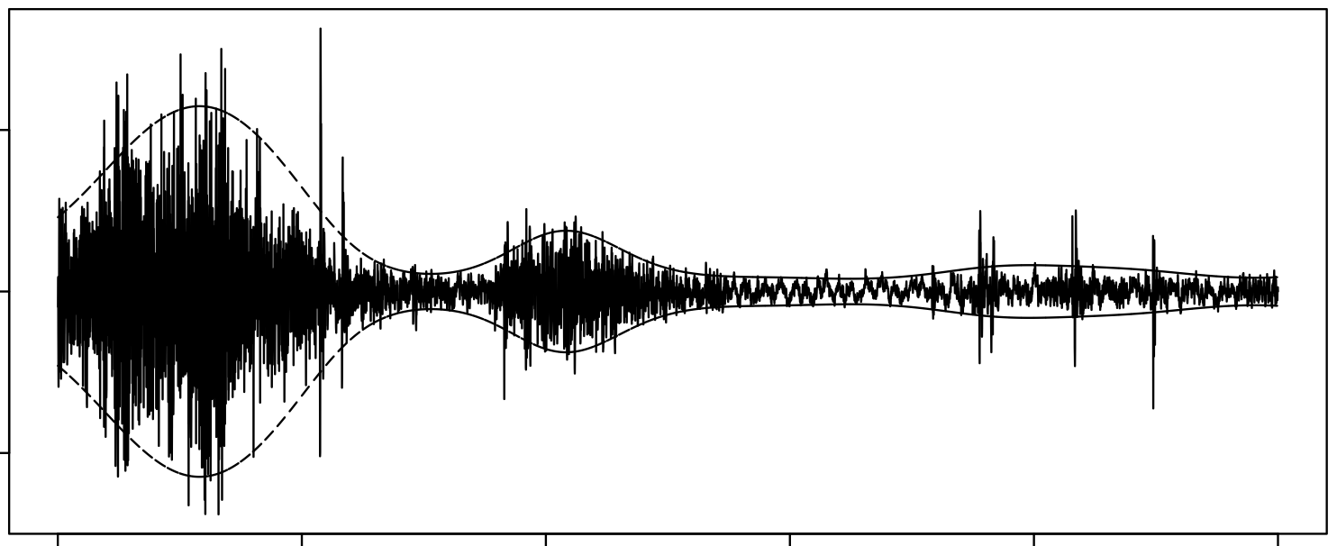
Modelling Audio using GPs
I used the S-PAD and the GP-PAD models from Richard Turner’s thesis to make these plots using some random audio data from the internet. These can be sense checked using rolling standard deviations.
Sample stan code for this.
// S-PAD
data {
	int n;     // len
	real x[n]; // audio
}
parameters {
	real<lower = 0, upper = 1> l;
	real<lower = 0, upper = 10> s;
	vector<lower = -10, upper = 2>[n] sigma;
}
model {
	sigma[1] ~ normal(0, s);
	sigma[2:n] ~ normal(l * sigma[1:(n - 1)], s*(1 - l^2)^0.5);
	x ~ normal(0, exp(sigma));
}

// GP-PAD
data {
	int n;
	int n_s; // nrow of S22
	real seg_a[n]; // audio sample
	matrix[n, n_s] factor; // mvn conditional distribution shift factor S12 * S22^(-1)
	cholesky_factor_cov[n_s] K22c; // cholesky factor of S22
}
parameters {
	real<lower = -7.5, upper = 10> mu;
	vector<lower = -7.5, upper = 10>[n_s] sigma;
}
transformed parameters {
	vector[n] sigma_vec;
	sigma_vec = rep_vector(mu, n) +
		factor*(sigma - rep_vector(mu, n_s));
}
model {
	sigma ~ multi_normal_cholesky(rep_vector(mu, n_s), K22c);
	seg_a ~ normal(0, log(1 + exp(sigma_vec)));
}
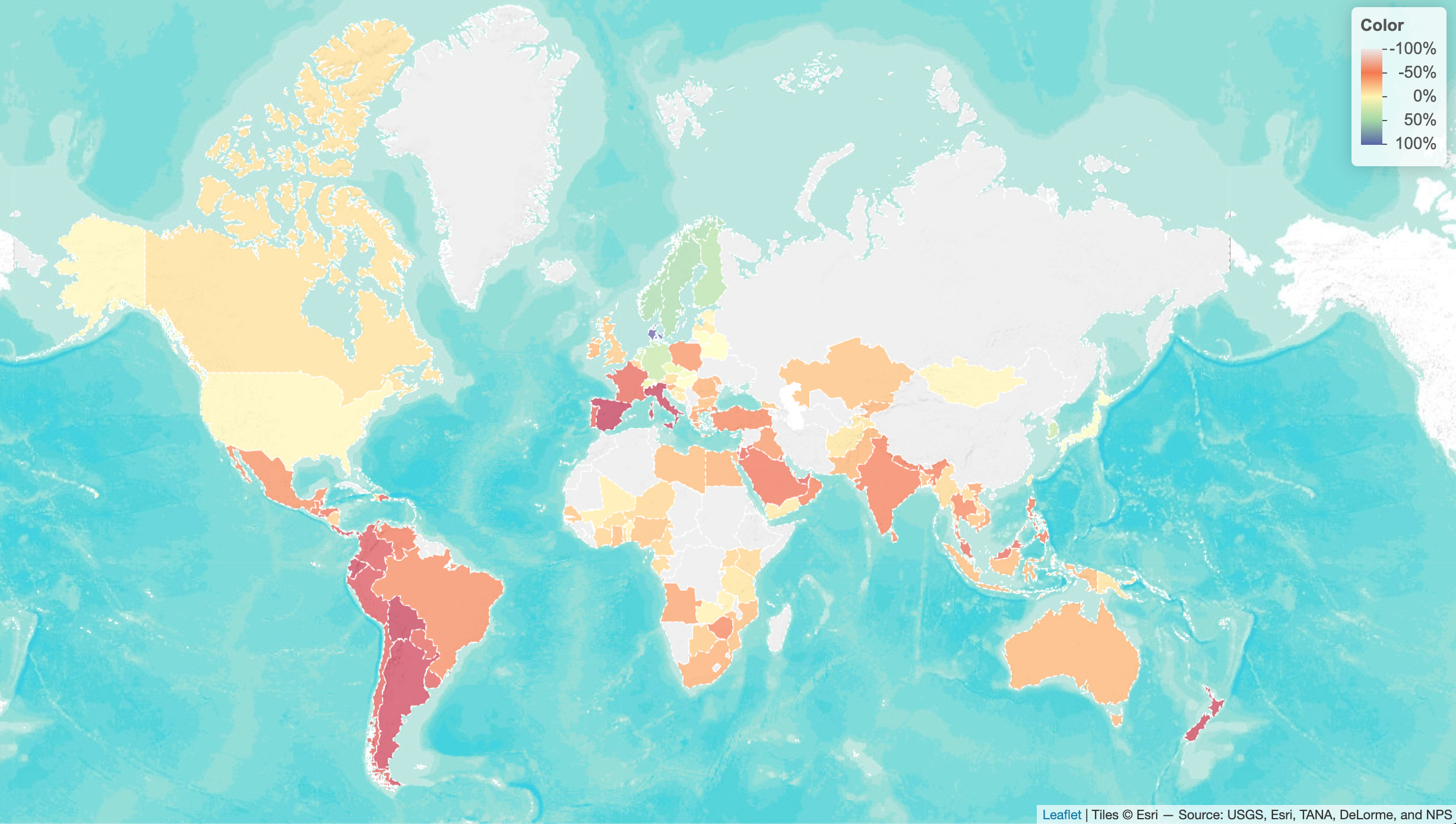
Changes in Park-Going
… w.r.t. baseline, as a result of the pandemic (as of 23rd Apr 2020). Based on the Google mobility dataset, plotted using leaflet.
2021
Efficient Gaussian Process Computation
Using einsum for vectorizing matrix ops
Gaussian Processes in MGCV
I lay out the canonical GP interpretation of MGCV’s GAM parameters here. Prof. Wood updated the package with stationary GP smooths after a request. Running through the predict.gam source code in a debugger, the computation of predictions appears to be as follows:
Short Side Projects
Snowflake GP
Photogrammetry
I wanted to see how easy it was to do photogrammetry (create 3d models using photos) using PyTorch3D by Facebook AI Research.
Dead Code & Syntax Trees
This post was motivated by some R code that I came across (over a thousand lines of it) with a bunch of if-statements that were never called. I wanted an automatic way to get a minimal reproducing example of a test from this file. While reading about how to do this, I came across Dead Code Elimination, which kills unused and unreachable code and variables as an example.
2020
Astrophotography
I used to do a fair bit of astrophotography in university - it’s harder to find good skies now living in the city. Here are some of my old pictures. I’ve kept making rookie mistakes (too much ISO, not much exposure time, using a slow lens, bad stacking, …), for that I apologize!
Probabilistic PCA
I’ve been reading about PPCA, and this post summarizes my understanding of it. I took a lot of this from Pattern Recognition and Machine Learning by Bishop.
Spotify Data Exploration
The main objective of this post was just to write about my typical workflow and views. The structure of this data is also outside my immediate domain so I thought it’d be fun to write up a small diary working with the data.
Random Stuff
For dealing with road/city networks, refer to Geoff Boeing’s blog and his amazing python package OSMnx. Go to Shapely for manipulation of line segments and other objects in python, networkx for networks in python and igraph for networks in R.
Morphing with GPs
The main aim here was to morph space inside a square but such that the transformation preserves some kind of ordering of the points. I wanted to use it to generate some random graphs on a flat surface and introduce spatial deformation to make the graphs more interesting.
SEIR Models
The model is described on the Compartmental Models Wikipedia Page.
Speech Synthesis
The initial aim here was to model speech samples as realizations of a Gaussian process with some appropriate covariance function, by conditioning on the spectrogram. I fit a spectral mixture kernel to segments of audio data and concatenated the segments to obtain the full waveform.
Sparse Gaussian Process Example
Minimal Working Example
2019
An Ising-Like Model
… using Stan & HMC
Stochastic Bernoulli Probabilities
Consider: