Introduction
The log-likelihood function \(l\) is a function such that:
\[\mathcal l(\theta; x) = ln \; p_{\mathcal M}(x|\theta)\]… where p is the generalized density under a model, evaluated on the dataset.
Model Laws
-
We can reason about the probability of failure in a repeated Bernoulli experiment even if no failures are observed! Assume that a process represented by \(X \sim Bin(n, p)\) produces a set of \(n\) successes. We can still construct a posterior by writing out the likelihood of this model. This would obviously include 0 (and the highest mass would be there) but an interval with a 5% error rate would be \([0, 3/n]\).
-
When dealing with censored data, we can re-frame the problem and derive a likelihood. Here’s my attempt at that:
Let a random variable \(\tau\) have a cumulative distribution function \(F_{\tau}\).
Now, let \(X\) be a random variable such that:
\[X = \begin{cases} \tau, & \text{if $\tau \leq T$} \\ T, & \text{if $\tau \geq T$} \end{cases}\]Then, it’s easy to see that the cumulative distribution function of \(X\) is:
\[F_X(x) = \begin{cases} F_{\tau}(x), & \text{if $x < T$} \\ 1, & \text{if $x \geq T$} \end{cases}\]Let \(\nu = l + \delta_T\) be a reference measure that is the sum of the Lebesgue measure \(l\) and the Dirac measure \(\delta_T\) on the set \(\{T\}\). Then, the density on \(X\) will be a function \(h\) (the Radon-Nikodym derivative) such that:
\[F_X(x) = \int_{-\infty}^x h d\nu = \int_{-\infty}^x h(u) du * \mathcal I_{x < T} + h(T) \mathcal I_{x = T}\]A function that satisfies the form above is:
\[h(u) = \frac{dF_{\tau}}{du}(u) \mathcal I_{u < T} + (1 - F_{\tau}(T)) \mathcal I_{u = T}\]
Dimensionality
Volumes in High Dimensions
A lot of probability theory uses the idea of volumes. For example, the probability and expectation are usually defined as:
\[\mathbb P_{\mu} (\mathcal A) = \int_A d \mu \;\;\; ; \;\;\; \mathbb E_{\mu} (f(X)) = \int_{\chi} f(x) d \mu(x)\]… where the differential element is usually a volume, \(d \mu(x) = p(x) dx_1 ... dx_d\), and p is a density, but volumes are really weird in higher dimensions.
The main idea is that our ideas of distance no longer make sense. Consider the following: I simulated a bunch of random normal points in many dimensions and plotted the average ratio of the distance to nearest point to the distance to farthest point:
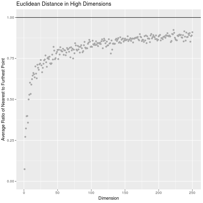
This ratio tends to one, implying that the nearest and farthest points are equally “close” / all points “look alike”.
On the same subject, consider a cube of unit lengths containing a sphere of unit radius in higher dimensions:


The edges of the cube keep more and more volume away from the sphere. In fact - the volume of a sphere starts decreasing after 5 dimensions.
Typical Sets
Consider the following: In one dimension, if I draw from a normal distribution, numbers close to zero would be the most reasonable guess at what the draw could be. In higher dimensions, this isn’t really the case - if I draw from a 1000-dimensional normal, it’s ridiculously unlikely that I’d pick a vector that (0, 0, 0, …); a more reasonable guess would be “a vector of points where the mean radius is ye much”.
Now consider the likelihood of an isolated repeated experiment:
\[L(\theta | x) = \prod_i^n p(x_i|\theta)\]This is a function of many random variables (which collectively have a dimension n). This will have it’s own sampling distribution, and the position where it’s maxmized w.r.t. any of the x’s isn’t a typical value of the likelihood at all.
Example:
hist_fancy(replicate(10000, sum(log(dnorm(rnorm(100))))),
           main = "Typical Values of the Loglikelihood", xlab = "ll")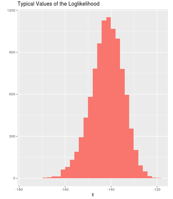
The maximum possible value of the loglikelihood in this case is -91.9, although it’s always much lower than that. Loglikelihood values around -140 for this experiment are typical.
We call values that lie in this region of typicality the typical set and it’s geometry is expected to be weird. From the other results, we expect it to be a thin layer of mass lying on a shell somewhere in a high dimensional space. The booklet “Logic, Probability, and Bayesian Inference” by Betancourt & the Stan Dev Team has another such example.
From Andrew Gelman’s blog: Interpolating between any two values of the typical set is rather unlikely to result in another typical sample. To sample from an arbitrary density, we can’t use grid or ensemble based methods, so a logical alternative is to start with a sample and obtain another sample using it, which leads logically to the idea of Markov Chain Monte Carlo, at which the Hybrid/Hamiltonian method is rather efficient.
R Code for Dimensionality Image
library(mvtnorm); library(ggplot2)

dim_dist <- function(d, samp_size = 10, ...){
	samp <- rmvnorm(samp_size, mean = rep(0, d), sigma = diag(1, d, d))
	dists <- as.matrix(dist(samp, diag = T, upper = T, ...))
	return(mean(sapply(1:samp_size, function(i) min(dists[-i, i])/max(dists[-i, i]))))
}

qplot(x = 1:250,
	  y = sapply(1:250, function(d) dim_dist(d)),
	  main = "Euclidean Distance in High Dimensions",
	  ylab = "Average Ratio of Nearest to Furthest Point",
	  xlab = "Dimension", color = I("dark gray"), ylim = c(0, 1)) +
	  geom_hline(aes(yintercept = 1))
2021
Efficient Gaussian Process Computation
Using einsum for vectorizing matrix ops
Gaussian Processes in MGCV
I lay out the canonical GP interpretation of MGCV’s GAM parameters here. Prof. Wood updated the package with stationary GP smooths after a request. Running through the predict.gam source code in a debugger, the computation of predictions appears to be as follows:
Short Side Projects
Snowflake GP
Photogrammetry
I wanted to see how easy it was to do photogrammetry (create 3d models using photos) using PyTorch3D by Facebook AI Research.
Dead Code & Syntax Trees
This post was motivated by some R code that I came across (over a thousand lines of it) with a bunch of if-statements that were never called. I wanted an automatic way to get a minimal reproducing example of a test from this file. While reading about how to do this, I came across Dead Code Elimination, which kills unused and unreachable code and variables as an example.
2020
Astrophotography
I used to do a fair bit of astrophotography in university - it’s harder to find good skies now living in the city. Here are some of my old pictures. I’ve kept making rookie mistakes (too much ISO, not much exposure time, using a slow lens, bad stacking, …), for that I apologize!
Probabilistic PCA
I’ve been reading about PPCA, and this post summarizes my understanding of it. I took a lot of this from Pattern Recognition and Machine Learning by Bishop.
Spotify Data Exploration
The main objective of this post was just to write about my typical workflow and views. The structure of this data is also outside my immediate domain so I thought it’d be fun to write up a small diary working with the data.
Random Stuff
For dealing with road/city networks, refer to Geoff Boeing’s blog and his amazing python package OSMnx. Go to Shapely for manipulation of line segments and other objects in python, networkx for networks in python and igraph for networks in R.
Morphing with GPs
The main aim here was to morph space inside a square but such that the transformation preserves some kind of ordering of the points. I wanted to use it to generate some random graphs on a flat surface and introduce spatial deformation to make the graphs more interesting.
SEIR Models
The model is described on the Compartmental Models Wikipedia Page.
Speech Synthesis
The initial aim here was to model speech samples as realizations of a Gaussian process with some appropriate covariance function, by conditioning on the spectrogram. I fit a spectral mixture kernel to segments of audio data and concatenated the segments to obtain the full waveform.
Sparse Gaussian Process Example
Minimal Working Example
2019
An Ising-Like Model
… using Stan & HMC
Stochastic Bernoulli Probabilities
Consider: